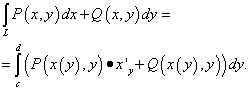
In case the integration area is a segment of some curve lying in the plane. General recording of the curvilinear integral as follows:

where f.(x., y.) - function of two variables, and L. - curve, by segment AB which integrates. If the integrand function is equal to one, then the curvilinear integral is equal to the length of the AB arc .

As always in integral calculus, the curvilinear integral is understood as the limit of integrated amounts of some very small parts of something very large. What is summed in the case of curvilinear integrals?

Let it be cut on the plane AB Some curve L., and the function of two variables f.(x., y.) Defined at the points of the curve L.. Let we carry out the following algorithm with this cut curve.

Split the curve AB Parts on the points (Pictures below).
In each part, to freely choose a point M..
Find the function in the selected points.
The values \u200b\u200bof the function multiply on
- the length of the parts in the case of curvilinear integral of the first kind ;
- projection parts on the coordinate axis in case the curvilinear integral of the second kind .
Find the sum of all works.
Find the limit of the found integrated amount, provided that the length of the longest part of the curve tends to zero.

If the mentioned limit exists, then this the limit of the integrated amount is called a curvilinear integral from the function f.(x., y.) By Krivoy AB .

First kind

Case of curvilinear integral
Second race

We introduce the following correspondence.

M.i ( ζ i; η i) - Selected point with coordinates on each site.

f.i ( ζ i; η i) - Function value f.(x., y.) In the selected point.

Δ s.i. - length of part of the segment of the curve (in the case of a curvilinear integral of the first kind).

Δ x.i. - Projection of part of the cutting curve on the axis OX. (in the case of a curvilinear integral of the second kind).

d. \u003d MaxΔ. s.i. - The length of the longest part of the cut curve.

The curvilinear integrals of the first kind

Based on the above-mentioned integrated amount, the curvilinear integral of the first kind is written as follows:

The curvilinear integral of the first kind has all the properties that possesses certain integral . However, there is one important difference. In a certain integral when changing places in places the integration limits, the sign changes to the opposite:

In the case of the curvilinear integral of the first kind, it does not matter what kind of curve points AB (A. or B.) consider the beginning of the segment, but which end, that is

Curvilinear integrals of the second kind

Based on the outlined integrated amount, the curvilinear integral of the second kind is written as:

In the case of a curvilinear integral of the second kind with a change in the start and end of the segment of the curve, the integral sign changes:

When compiling the integrated amount of the curved integral of the second kind of function value f.i ( ζ i; η i) You can also multiply on the projection of the parts of the segment of the curve on the axis Oy.. Then we get an integral

In practice, it is usually used to combine the curvilinear integrals of the second kind, that is, two functions f. = P.(x., y.) and f. = Q.(x., y.) and integrals

and the sum of these integrals

called common curvilinear integral of the second kind .

Calculation of curvilinear integrals of the first kind

The calculation of the curvilinear integrals of the first kind is reduced to the calculation of certain integrals. Consider two cases.

Let the plane set the curve y. = y.(x.) and cutting curve AB corresponds to change variable x. from a. before b.. Then at the point of the curve, the integrand function f.(x., y.) = f.(x., y.(x.)) ("igrek" should be expressed through "X"), and the differential of the arc and curvilinear integral can be calculated by the formula

If the integral is easier to integrate by y.then from the equation of the curve you need to express x. = x.(y.) ("Iks" through "Igrek"), where and the integral calculate the formula

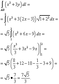
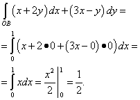
Example 1.

where AB - cut straight between dots A.(1; -1) and B.(2; 1) .

Decision. Make an equation direct AB Using the formula (equation direct passing through two points data A.(x.1 ; y.1 ) and B.(x.2 ; y.2 ) ):

From the equation to express y. through x. :

Then and now we can calculate the integral, since we have some "Ikers" left:

Let the curve aspass in space

Then at the point of the curve, the function must be expressed through the parameter t. () And Differential Arc , so the curvilinear integral can be calculated by the formula

Similarly, if the plane is given a curve

then the curvilinear integral is calculated by the formula

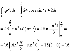
Example 2. Calculate the curvilinear integral

where L. - part of the circle line

located in the first octant.

Decision. This curve is a quarter line of the circle lines located in the plane z. \u003d 3. It corresponds to the parameter values. As

then Dougie Differential

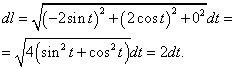
Integrated function express through the parameter t. :

Now that everything is pronounced through the parameter t. , We can reduce the calculation of this curvilinear integral to a specific integral:

Calculation of curvilinear integrals of the second kind

Also, as in the case of curvilinear integrals of the first kind, the calculation of the integrals of the second kind is reduced to the calculation of certain integrals.

Curve Dana in Cartesian rectangular coordinates

Let it be given a curve on the plane by the equation of the "Cheerk" function, expressed through "X": y. = y.(x.) and arc krivoy AB corresponds to change x. from a. before b. . Then in the integrated function we will substitute the expression "Games" through "X" and we define the differential of this expression "Games" on "ICSU" :. Now that everything is expressed through "X", the curvilinear integral of the second kind is calculated as a specific integral:

Similarly, the curvilinear integral of the second kind is calculated when the curve is given by the equation of the "X" function, expressed through "Igrek": x. = x.(y.) . In this case, the formula for calculating the integral is as follows:

Example 3. Calculate the curvilinear integral

, if a

but) L. - Straight cut Oa. where ABOUT(0; 0) , A.(1; −1) ;

b) L. - Arc parabola y. = x.² OT ABOUT(0; 0) to A.(1; −1) .

a) Calculate the curvilinear integral in a straight line (in the figure - blue). We will write the equation direct and express "Ix" through "X":

Receive dY. = dX. . We solve this curvilinear integral:

b) if L. - Arc parabola y. = x.², we get dY. = 2xDX . Calculate the integral:

In the one and the same result, the same result was obtained in two cases. And this is not a coincidence, but the result of regularity, since this integral satisfies the conditions of the following theorem.

Theorem. If functions P.(x.,y.) , Q.(x.,y.) and their private derivatives - continuous in the area D. functions and points of this area of \u200b\u200bprivate derivatives are equal, then the curvilinear integral does not depend on the path integration path L. located in the field D. .

The curve is given in parametric form

Let in space given a curve

and in the integrative functions we will substitute

expressions of these functions through the parameter t. . We get a formula for calculating a curvilinear integral:

Example 4. Calculate the curvilinear integral

if a L. - Part of the ellipse

conducting condition y. ≥ 0 .

Decision. This curve is part of the ellipse in the plane z. \u003d 2. It corresponds to the value of the parameter.

we can submit a curvilinear integral in the form of a specific integral and calculate it:

If the curvilinear integral and L. - a closed line, then such an integral is called an integral over a closed circuit and it is easier to calculate green formula .

More examples of calculating curvilinear integrals

Example 5. Calculate the curvilinear integral

where L. - Cut the line between its intersection points with the coordinate axes.

Decision. We define the intersection points of the line with the axes of coordinates. Substituting in the direct equation y. \u003d 0, we get. Substation x. \u003d 0, we get. Thus, the point of intersection with the axis OX. - A.(2; 0), with axis Oy. - B.(0; −3) .

From the equation to express y. :

, .

Now we can present a curvilinear integral in the form of a certain integral and start calculating it:

In the integrand, we allocate the multiplier, we endure it for the sign of the integral. In the resulting initial expression apply summing up a differential sign And finally get.

Calculation of the curvilinear integral by coordinates.

Calculating the curvilinear integral by coordinates to reduce the calculation of an ordinary specific integral.

Consider the curvilinear integral of the 2nd order under the arc:

(1)

Let the integration curve equation specified in parametric form:

where t. - parameter.

Then from equations (2) we have:

Of the same equations recorded for points BUT and IN,

find values t. A. and t. B. parameters corresponding to the beginning and end of the integration curve.

Substitting the expression (2) and (3) to the integral (1), we obtain a formula for calculating the curvilinear integral of the 2nd kind:

If the integration curve is given explicitly relative to the variable y.. as

y \u003d f (x), (6)

then take a variable x. for parameter (t \u003d x) And we obtain the following entry of equation (6) in parametric form:

From here we have: , t. A. \u003d X. A. , t. B. \u003d X. B. , and curvilinear integral of the 2nd lead to a specific integral in a variable x.:

where y (x) - The equation of the line of which is integrating.

If the integration curve equation AU specified in explicit form relative to the variable x.. as

x \u003d φ (y) (8)

we will take for the variable parameter y., Write equation (8) in parametric form:

We get: , t. A. \u003d y. A. , t. B. \u003d y. B. , and the formula for calculating the integral of the 2nd kind takes the form:

where x (y) - line equation AU.

Comments.

one). The curvilinear integral in coordinates exists, i.e. There is a finite integrated amount when n.→∞ if on the function integration curve P (x, y)and Q (X, Y) continuous, and functions x (t) and y (t) Continuous together with their first derivatives and.

2). If the integration curve is closed, then you need to follow the direction of integration, since

Calculate integral , if a AU Set by equations:

but). (X-1) 2 + y. 2 =1.

b). y \u003d X.

in). y \u003d X. 2

Case A. Integration Line is the circle of radius R \u003d 1. with center at point C (1; 0). Its parametric equation:

Find

Determine the values \u200b\u200bof the parameter t. At points BUT and IN.

Point A. t. A. =π .

Case B. Parabola integration line. Accept x. For parameter. Then ,,

We get:

Green formula.

The Green Formula establishes the link between the curvilinear integral of the 2nd kind on a closed contour and a double integral in the area D.limited to this contour.

If the function P (x, y) and Q (X, Y) and their private derivatives and continuous in the area D.limited contour L., then there is a formula:

(1)

- Green formula.

Evidence.

Consider in the plane xoy. region D.correct in the direction of coordinate axes OX.and Oy..

TO oNTUR L. straight x \u003d A.and x \u003d B. divided into two parts, on each of which y. is an unambiguous function from x.. Let the upper part Ad. The contour is described by the equation y \u003d y. 2 (x), and lower plot QA Contour - equation y \u003d y. 1 (x).

Consider a double integral

Considering that the internal integral is calculated when x \u003d const. We get:

But the first integral in this amount, as follows from formula (7), is a curvilinear line integral VDA, as y \u003d y. 2 (x) - equation of this line, i.e.

and the second integral is a curvilinear integral function P (x, y) on line QA, as y \u003d y. 1 (x) - equation of this line:

The sum of these integrals is a curvilinear integral over a closed contour L. from function P (x, y) By coordinate x..

As a result, we get:

(2)

After splitting L. straight y \u003d C. and y \u003d D. On the plots GARDEN and SVDdescribed according to equations x \u003d X. 1 (y) and x \u003d X. 2 (y.) Similarly, we get:

Folding the right and left parts of equals (2) and (3), we obtain the Green formula:

Corollary.

Using the curvilinear integral of the 2nd genus, it is possible to calculate the area of \u200b\u200bflat figures.

We define how functions should be P (x, y)and Q (X, Y). We write:

or, applying the Green formula,

Consequently, equality should be performed

what perhaps, for example,

Where do you get:

(4)

Calculate the area bounded by the ellipse, the equation of which is set in parametric form:

The condition of independence of the curvilinear integral coordinates from the path of integration.

We found that according to the mechanical meaning, the curvilinear integral of the 2nd genus represents the operation of a variable force on the curvilinear path or in other words, work on moving the material point in the field. But from physics, it is known that work in the field of gravity does not depend on the form of the path, but depends on the position of the initial and endpoint points. Therefore, there are cases when the curvilinear integral of the 2nd kind does not depend on the path of integration.

We define the conditions under which the curvilinear integral in coordinates does not depend on the path of integration.

Let in some region D. Functions P (x, y) and Q (X, Y) and private derivatives

And continuous. Take in this area of \u200b\u200bthe point BUT and IN and connect them arbitrary lines QA and AFB..

If the curvilinear integral of the 2nd kind does not depend on the path of integration, then

(1)

But the integral (1) is an integral on a closed contour ACBFA..

Consequently, the curvilinear integral of the 2nd kind in some region D. It does not depend on the path of integration if the integral on any closed contour in this area is zero.

We define what conditions must satisfy the functions P (x, y) and Q (X, Y) In order for equality

, (2)

those. In order for the curvilinear integral in coordinates does not depend on the path of integration.

Let in the area D. Functions P (x, y) and Q (X, Y) And their private derivatives of the first order and are continuous. Then in order for the curvilinear integral by coordinates

did not depend on the path of integration, it is necessary and enough to in all points of the region D. Equality was performed

Evidence.

Consequently, equality is performed (2), i.e.

, (5)

for which it is necessary to fulfill the condition (4).

Then, from equation (5) it follows that equality (2) is performed and, therefore, the integral does not depend on the path of integration.

Thus, the theorem is proved.

We show that the condition

performed if the integrand

is a complete differential of any function U (x, y).

The full differential of this function is equal

. (7)

Let the integrand (6) be a complete differential function U (x, y).

from where it follows that

Of these equations, we find expressions for private derivatives and:

, .

But the second mixed private derivatives do not depend on the procedure for differentiation, therefore, it was necessary to prove. curvilinear integrals. You should also ... applications. From theory curvilinear integrals it is known that curvilinear integral of the form (29 ...

Differential calculus of the function of one variable

Abstract \u003e\u003e Mathematics

... (Ed2) Finding Square curvilinear Sectors.  \u003d f ()     To find the area curvilinear Sectors We introduce a polar ... gradient with a derivative direction. Multiples integrals. Double integrals. The conditions for the existence of a double integral. Properties ...

Implementation of mathematical models using integration integration methods in Matlab

Coursework \u003e\u003e Computer Science

... (i \u003d 1.2, ..., n). Fig. 5 - Formula of the trapezium Then area krivolyinene The trapezoids bounded by the lines x \u003d a, x \u003d b, y \u003d 0, y \u003d f (x), and therefore (following ... in character form are calculated by any multiples integrals. 2. Matlab - Matlab modeling environment (Matrix ...

Actions with approximate values

Abstract \u003e\u003e Mathematics

Various equations, and when calculating certain integralsand in the approximation of the function. Consider various methods ...  x2 ...  xk + m. In the k equation multiple and m internally multiple roots. It is declined to (k + m) equations ...

If a curvilinear integral is given, and the curve at which integrating is closed (called the contour), then such an integral is called an integral over a closed circuit and is indicated as follows:

Contour L. Denote D.. If functions P.(x., y.) , Q.(x., y.) and their private derivatives and - functions continuous in the area D., To calculate the curvilinear integral, you can use the Green Formula:

Thus, the calculation of the curvilinear integral on a closed contour is reduced to the calculation of the double integral in the region D..

The Green Formula remains fair for any closed area, which can be carried out by additional lines to a finite number of simple closed regions.

Example 1. Calculate the curvilinear integral

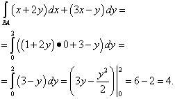
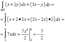
if a L. - Contour of the triangle OAB where ABOUT(0; 0) , A.(1; 2) and B.(10) . Direction of circuit crawl - counterclockwise. The task is to solve in two ways: a) calculate curvilinear integrals on each side of the triangle and fold the results; b) according to the Green formula.

a) Calculate curvilinear integrals on each side of the triangle. Side OB. Located on the axis OX. , so its equation will be y. \u003d 0. therefore dY. \u003d 0 and can calculate the curvilinear integral by side OB. :

Part side equation BA. will be x. \u003d 1. therefore dX. \u003d 0. Calculate the curvilinear integral on the side BA. :

Partway equation AO. We will make using the formula of the equation direct passing in two points:

In this way, dY. = 2dX. . Calculate the curvilinear integral on the side AO. :

This curvilinear integral will be equal to sum Integrals on the edges of the triangle:

b) Apply Green's formula. As , T. . We have everything in order to calculate this integral on a closed contour by the Green formula:

As we can see, the same result was obtained, but according to the Green formula, the calculation of the integral on a closed contour is much faster.

Example 2.

where L. - contour OAB , OB. - Arc parabola y. = x.², from point ABOUT(0; 0) to the point A.(1; 1) , AB and BO. - straight cuts, B.(0; 1) .

Decision. As functions, and their private derivatives ,, D. - area limited by contour L. We have everything to take advantage of the Green formula and calculate this integral on a closed contour:

Example 3. Using the Green Formula, calculate the curvilinear integral

, if a L. - contour that form the line y. = 2 − |x.| and axis Oy. .

Decision. Line y. = 2 − |x.| Consists of two rays: y. = 2 − x. , if a x. ≥ 0 I. y. = 2 + x. , if a x. < 0 .

We have functions, and their private derivatives and. We substitute everything in the Green formula and get the result.

Department " Higher mathematics»

Curvilinear integrals

Methodical instructions

Volgograd

UDC 517.373 (075)

Reviewer:

senior Lecturer of the Department "Applied Mathematics" N.I. Koltsova

Printed by the decision of the editorial and publishing council

Volgograd State Technical University

Curvilinear integrals: method. Indications / Sost. M.I. Andreeva,

O.E. Grigoriev; VolgGTU. - Volgograd, 2011. - 26 p.

Methodical instructions are a guide to the implementation of individual tasks on the topic "Curvoline integrals and their applications to the field theory".

The first part of the guidelines contains the necessary theoretical material for the implementation of individual tasks.

In the second part, examples of the implementation of all types of tasks included in individual tasks on the topic, which contributes to the best organization independent work Students and successful assimilation of the topic.

Methodical instructions are designed for students of the first and second courses.

technical University, 2011

Curvilinear integral 1 kind

Determination of the curvilinear integral 1 kind

Let è. AU - arc flat or spatial piecewise smooth curve L., f.(P.) - asked on this arc continuous function, BUT 0 = BUT, BUT 1 , BUT 2 , …, A N. – 1 , A N. = B. AU and P I. - Arbitrary points on partial arcs è A I. – 1 A I., whose lengths D l I. (i. = 1, 2, …, n.

for n. ® ¥ and MAX D l I. ® 0, which does not depend on the way of splitting the arc è AU Points A I.nor from choosing points P I. on partial arcs è A I. – 1 A I. (i. = 1, 2, …, n.). This limit is called a curvilinear integral of 1 kind from the function f.(P.) By Krivoy L. And denotes

Calculation of curvilinear integral 1 kind

The calculation of the curvilinear integral 1 of the genus may be reduced to the calculation of a specific integral with different ways of setting the integration curve.

If the arc è. AU a flat curve is set by parametric equations where x.(t.) I. y.(t. t., and x.(t. 1) = x A., x.(t. 2) = x B.T.

where - Differential of the length of the arc curve.

A similar formula takes place in the case of a parametric task of a spatial curve L.. If the arc è. AUcrooked L.set by equations and x.(t.), y.(t.), z.(t.) - continuously differentiable parameter functions t.T.

where - differential the length of the arc curve.

in cartesian coordinates

If the arc è. AU flat curve L. Posted by equation Where y.(x.

and the formula for calculating the curvilinear integral has the form:

When specifying arc è AU flat curve L. as x.= x.(y.), y. Î [ y. 1 ; y. 2 ],
Where x.(y.) - continuously differentiable function,

and curvilinear integral is calculated by the formula

(1.4)

Setting the integration curve by the polar equation

If flat curve L. set by the equation in the polar coordinate system r. = r.(j), j î, where r.(j) - continuously differentiable function, then

and

(1.5)

Applications of the curvilinear integral 1 kind

With the help of a curvilinear integral 1 of the genus calculated: the length of the arc curve, the area of \u200b\u200bthe cylindrical surface, mass, static moments, moments of inertia and the coordinates of the center of gravity material curve with a given linear density.

1. Length l. flat or spatial curve L.located by formula

2. Area of \u200b\u200ba cylindrical surface with parallel axis Oz. forming and located in the plane Xoy. Guide L.concluded between the plane Xoy. and the surface defined by the equation z. = f.(x.; y.) (f.(P.) ³ 0 when P. Î L.), equal

(1.7)

3. Massa m. material curve L. with linear density M ( P.) Formula is determined

(1.8)

4. Static moments relative to the axes OX. and Oy. and coordinates of the center of gravity flat material curve L.with linear density M ( x.; y.) are equal, respectively:

(1.9)

5. Static moments relative to the planes Oxy, Oxz., Oyz. and coordinates of the center of gravity of a spatial material curve with a linear density M ( x.; y.; z) are determined by formulas:

(1.11)

6. For a flat material curve L. with linear density M ( x.; y.) moments of inertia relative to the axes OX., Oy. and the start of coordinates are respectively equal:

(1.13)

7. Moments of inertia spatial material curve L. with linear density M ( x.; y.; z) relative to the coordinate planes are calculated by formulas

(1.14)

and moments of inertia relative to the coordinate axes are equal:

(1.15)

2. Krivolynoe integral 2 kind

Determination of the curvilinear integral of 2 kind

Let è. AU - arc piecewise and smooth oriented curve L., = (a X.(P.); a Y.(P.); a Z.(P.)) - a continuous vector function specified on this arc, BUT 0 = BUT, BUT 1 , BUT 2 , …, A N. – 1 , A N. = B. - arbitrary splitting of the arc AU and P I. - arbitrary points on partial arcs A I. – 1 A I.. Let - the vector with coordinates D x I., D. y I., D. z I.(i. = 1, 2, …, n.), and - scalar product vectors and ( i. = 1, 2, …, n.). Then there is a limit of the sequence of integrated amounts

for n. ® ¥ and max ÷ ç® 0, which does not depend on the way of splitting an arc AU Points A I.nor from choosing points P I. on partial arcs è A I. – 1 A I.
(i. = 1, 2, …, n.). This limit is called a curvilinear integral of 2 genus from the function ( P.) By Krivoy L. And denotes

In the case when the vector function is set on a flat curve L.Similarly, we have:

When the integration direction is changed, the curvilinear integral of 2 generates changes the sign.

The curvilinear integrals of the first and second kind are associated with the relation

(2.2)

where is the single vector tangent to the oriented curve.

Using a curvilinear integral of 2 kinds, it is possible to calculate the work of force when moving the material point along the arc of the curve L:

(2.3)

Positive direction by closed curve FROM,recognizing a single-connected area G.The following is to be around counterclockwise.

Curvilinear integral 2 kind of closed curve FROM called circulation and denoted

(2.4)

Calculation of curvilinear integral 2 kind

Calculation of the curvilinear integral of 2 types is reduced to calculating a specific integral.

Parametric task of integration curve

If è. AU The oriented flat curve is set by parametric equations where h.(t.) I. y.(t.) - continuously differentiable parameter functions t., and that

(2.5)

A similar formula takes place in the case of a parametric task of a spatial oriented curve L.. If the arc è. AUcrooked L. set by equations and - continuously differentiable parameter functions t.T.

(2.6)

Explicit task of a flat integration curve

If the arc è. AU L. set in the Cartesian coordinates by the equation where y.(x.) - continuously differentiable function, then

(2.7)

When specifying arc è AUflat oriented curve L. as
x.= x.(y.), y. Î [ y. 1 ; y. 2] where x.(y.) - continuously differentiable function, the formula is valid

(2.8)

Let functions continuous with their derivatives

in a flat closed area G.limited by a piecewise smooth closed self-moving positively oriented curve FROM +. Then the Green Formula is:

Let be G. - Single-connected area, and

= (a X.(P.); a Y.(P.); a Z.(P.))

- set in this area vector field. Field ( P.) is called potential if there is such a function U.(P.), what

(P.) \u003d Grad. U.(P.),

I. sufficient condition potentiality of vector field ( P.) It looks:

rot ( P.) \u003d, where (2.10)

(2.11)

If the vector field is potential, then the curvilinear integral of 2 kind does not depend on the integration curve, and depends only on the coordinates of the beginning and end of the arc M. 0 M.. Potential U.(M.) The vector field is determined with an accuracy of the constant component and is located by the formula

(2.12)

where M. 0 M. - arbitrary curve connecting a fixed point M. 0 and variable point M.. To simplify computing as a path of integration can be selected broken M. 0 M. 1 M. 2 M. With links parallel to the coordinate axes, for example:

3. Examples of tasks

Exercise 1

Calculate the curvilinear integral of the genus

where L is an arc of curve, 0 ≤ x. ≤ 1.

Decision.According to the formula (1.3), the information of the curvilinear integral of the genus to a specific integral in the case of a smooth flat clearly specified curve:

where y. = y.(x.), x. 0 ≤ x. ≤ x. 1 - arc equation L. integration curve. In this example Find a derivative of this function

and differential curve arc length L.

then putting into this expression instead y.Receive

We transform a curvilinear integral to a specific:

Calculate this integral by substitution. Then
t. 2 = 1 + x., x. = t. 2 – 1, dX. = 2t dt.; for x \u003d. 0 t. \u003d 1; but x. \u003d 1 corresponds. After transformation, we get

Task 2.

Calculate curvilinear integral 1 kind Around L. crooked L.: X. \u003d COS 3. t., y. \u003d SIN 3. t., .

Decision. As L. - an arc of a smooth flat curve given in parametric form, we use formula (1.1) the information of the curvilinear integral of 1 to the specified:

In this example

Find the Differential of the length of the arc

Found expressions we substitute in formula (1.1) and calculate:

Task 3.

Find a lot of arc lines L. With a linear plane m.

Decision. Weight m.dougi. L. with density M ( P.) is calculated by formula (1.8)

This is a curvilinear integral of 1 of the genus over a parametrically defined smooth arc curve in space, therefore it is calculated by the formula (1.2) of the information of the curvilinear integral 1 of the genus to a specific integral:

We find derivatives

and Differential Arc length

We substitute these expressions in the mass formula:

Task 4.

Example 1. Calculate curvilinear integral 2 kind

around L.curve 4. x. + y. 2 \u003d 4 from the point A.(1; 0) to the point B.(0; 2).

Decision. Flat arc L. set in implicit form. To calculate the integral, it is more convenient to express x. through y.:

and find an integral according to formula (2.8) converting a curvilinear integral of 2 kind to a specific integral by variable y.:

where a X.(x.; y.) = xY. – 1, a Y.(x.; y.) = xY. 2 .

Taking into account the task of the curve

By formula (2.8) we get

Example 2.. Calculate curvilinear integral 2 kind

where L. - Loars ABC, A.(1; 2), B.(3; 2), C.(2; 1).

Decision. By the property of the additivity of the curvilinear integral

Each of the integral-terms calculate the formula (2.7)

where a X.(x.; y.) = x. 2 + y., a Y.(x.; y.) = –3xY..

The cut equation is direct AB: y. = 2, y.¢ = 0, x. 1 = 1, x. 2 \u003d 3. Substituting these expressions in formula (2.7), we obtain:

To calculate the integral

make an equation direct BC. according to the formula

where x B., y B., x C., y C - coordinates of the point B. and FROM. Receive

y. – 2 = x. – 3, y. = x. – 1, y.¢ \u003d 1.

We substitute the obtained expressions in formula (2.7):

Task 5.

Calculate curvilinear integral 2 kind of arc L.

0 ≤ t. ≤ 1.

Decision. Since the integration curve is set by parametric equations x \u003d X.(t.), y \u003d y.(t.), t. Î [ t. 1 ; t. 2] where x.(t.) I. y.(t.) - continuously differentiable functions t. for t. Î [ t. 1 ; t. 2], then for calculating the curvilinear integral of the second kind, we use formula (2.5) information of the curvilinear integral to a defined parameter-defined curve

In this example a X.(x.; y.) = y.; a Y.(x.; y.) = –2x..

C for the purpose of the task of the curve L. We get:

We substitute the found expressions in formula (2.5) and calculate a specific integral:

Task 6.

Example 1. C. + Where FROM : y. 2 = 2x., y. = x. – 4.

Decision. Designation C. + Indicates that the contour bypass is carried out in the positive direction, that is, counterclockwise.

Check that the Green formula (2.9) can be used to solve the problem.

Since functions a X. (x.; y.) = 2y. – x. 2 ; a Y. (x.; y.) = 3x. + y. and their private derivatives Continuous in flat closed area G.limited contour C., Tormula Green is applicable.

To calculate the double integral, depict the area G., pre-determining the intersection points of the arc curves y. 2 = 2x. and
y. = x. - 4 constituent contour C..

The intersection points will find by solving the system of equations:

The second equation of the system is equivalent to equation x. 2 – 10x. + 16 \u003d 0, from where x. 1 = 2, x. 2 = 8, y. 1 = –2, y. 2 = 4.

So, the intersection points of the curves: A.(2; –2), B.(8; 4).

Since the area G.- Right in the direction of the axis OX., then for the information of the double integral to re-describe the area G. on the axis Oy. And we use the formula

As a. = –2, b. = 4, x. 2 (y.) = 4+y.T.

Example 2. Calculate curvilinear integral 2 kind on closed contour Where FROM - Contour of the triangle with vertices A.(0; 0), B.(1; 2), C.(3; 1).

Decision. The designation means that the contour of the triangle costs clockwise. In the case when the curvilinear integral is taken over a closed contour, the Green formula takes the view

Show area G.limited by the specified contour.

Functions and private derivatives and Continuous in the area G.Therefore, you can apply Green's formula. Then

Region G. It is not correct towards any of the axes. We carry out the cut straight x. \u003d 1 and imagine G. as G. = G. 1 è. G. 2, where G. 1 I. G. 2 areas correct in the direction of the axis Oy..

Then

For each of the double integrals by G. 1 I. G. 2 to repeat the formula

where [ a.; b.] - Projection of the region D. on the axis OX.,

y. = y. 1 (x.) - the equation of the lower bounding curve,

y. = y. 2 (x.) - The equation of the upper limiting curve.

We write the equations of the boundaries of the region G. 1 and find

AB: y. = 2x., 0 ≤ x. ≤ 1; AD: , 0 ≤ x. ≤ 1.

Make an equation of the border BC. Region G. 2 using the formula

BC.: where 1 ≤ x. ≤ 3.

DC: 1 ≤ x. ≤ 3.

Task 7.

Example 1. Find the work of power L.: y. = x. 3 from the point M.(0; 0) to the point N.(1; 1).

Decision. The operation of variable force when moving the material point on the arc of the curve L. Determine by formula (2.3) (as a curvilinear integral of the second kind from the curve function L.) .

Since the vector function is set by the equation and arc of a flat-oriented curve is determined explicitly by the equation y. = y.(x.), x. Î [ x. 1 ; x. 2] where y.(x.) continuously differentiable function, then according to formula (2.7)

In this example y. = x. 3 , , x. 1 = x M. = 0, x. 2 = x N. \u003d 1. Therefore

Example 2.. Find the work of power When moving the material point along the line L.: x. 2 + y. 2 \u003d 4 from the point M.(0; 2) to the point N.(–2; 0).

Decision. Using formula (2.3), we get

In the example of an arc of the curve L.(È MN.) - this is a quarter of the circle defined by the canonical equation x. 2 + y. 2 = 4.

To calculate the curvilinear integral of the second kind, it is more convenient to move to the parametric task of the circle: x. = R.cos. t., y. = R. sin. t. and take advantage of Formula (2.5)

As x. \u003d 2cos. t., y. \u003d 2sin t., , Receive

Task 8.

Example 1.. Calculate vector field circulation module Along the contour G.:

Decision. To calculate the circulation of vector field along a closed contour G. We use formula (2.4)

Since the spatial vector field is set and spatial closed circuit G., passing from the vector form of writing a curvilinear integral to the coordinate form, get

Curve G. As the intersection of two surfaces is given: hyperbolic paraboloid z \u003d X. 2 – y. 2 + 2 and cylinder x. 2 + y. 2 \u003d 1. To calculate the curvilinear integral, it is convenient to switch to parametric curve equations G..

The cylindrical surface equation can be written in the form:
x. \u003d COS. t., y. \u003d SIN t., z. = z.. Expression for z. In parametric equations, the curve is obtained by substitution x. \u003d COS. t., y. \u003d SIN t. in the hyperbolic paraboloid equation z \u003d. 2 + COS 2 t. - SIN 2. t. \u003d 2 + COS 2 t.. So, G.: x. \u003d COS. t.,
y. \u003d SIN t., z. \u003d 2 + COS 2 t., 0 ≤ t. ≤ 2p.

Since curve included in parametric equations G. Functions
x.(t.) \u003d COS. t., y.(t.) \u003d sin. t., z.(t.) \u003d 2 + COS 2 t. are continuously differentiable parameter functions t. for t. Î, then the curvilinear integral is found according to formula (2.6)

The calculation of the volume is more convenient to lead in cylindrical coordinates. Equation of a circle bounding domain, cone and paraboloid

accordingly, they take the form ρ \u003d 2, z \u003d ρ, z \u003d 6 - ρ 2. Taking into account the fact that this body is symmetrically relative to the XOZ and Yoz planes. have

	6- ρ 2.
	6- ρ 2.
V \u003d 4 ∫ 2 dφ ∫ ρ dρ ∫ dz \u003d 4 ∫ 2 dφ ∫ ρ z		6 ρ - ρ 2 D ρ \u003d

4 ∫ D φ∫ (6 ρ - ρ3 - ρ2) d ρ \u003d

2 D φ \u003d

4 ∫ 2 (3 ρ 2 -

∫ 2 D φ \u003d

32π.

If not to take into account symmetry, then

6- ρ 2.

32π.

V \u003d ∫

dφ ∫ ρ dρ ∫ dz \u003d

3. Curvoline integrals

A summary of the concept of a certain integral in case the integration area is some curve. Integrals of this kind are called curvilinear. There are two types of curvilinear integrals: curvilinear integrals in length of arc and curvilinear integrals by coordinates.

3.1. Determination of the curvilinear integral of the first type (along the length of the arc). Let the function f (x, y) be determined along flat piecewise

smooth1 curve L, the ends of which will be points a and b. We divide the curve l randomly on the N parts of the points M 0 \u003d A, M 1, ... M n \u003d b. On the

each of the partial arcs M i m i + 1 will choose an arbitrary point (X I, Y i) and calculate the values \u200b\u200bof the function f (x, y) in each of these points. Sum

1 The curve is called a smooth, if at each it point there is a tangent, continuously changing along the curve. A pieting curve is a curve consisting of a finite number of smooth pieces.

n - 1.
Σ n \u003d σ f (x i, y i) Δ l i,

i \u003d 0.

whereΔ L i is the length of the partial arc M i m i + 1, called integral sum

for the function f (x, y) by curve L. Denote the greatest length
partial arc M i m i + 1, i \u003d
	0, n - 1 throughλ, that is, λ \u003d max Δ L i.
		0 ≤i ≤n -1
If there is a finite limit of the I integral sum (3.1)
the desire to zero the greatest of the length of the partial arcm i m i + 1,
depending on the method of splitting the curve L on partial arcs or from

selection of points (x i, y i), then this limit is called curvilinear integral of the first type (curvilinear integral in length of the arc)from the function f (x, y) by curve L and is denoted by the symbol ∫ F (x, y) DL.

Thus, by definition
Thus, by definition
n - 1.
I \u003d Lim Σ F (xi, yi) Δ li \u003d ∫ f (x, y) dl.
λ → 0 i \u003d 0

Function f (x, y) is called in this case integrated along the curveL,

the curve L \u003d AB is a circuit of integration, a - initial, and in - the end points of integration, DL - an element of the arc length.

Note 3.1. If in (3.2) put f (x, y) ≡ 1 for (x, y) l, then

we obtain the expression of the length of the arc L in the form of the curvilinear integral of the first type

l \u003d ∫ DL.


Indeed, from the definition of a curvilinear integral follows
	dL \u003d LIM N - 1
	dL \u003d LIM N - 1	ΔL.	LIM L \u003d L.
	λ → 0 ∑		λ→ 0
	i \u003d 0.

3.2. The main properties of the curvilinear integral of the first type
similar properties of a specific integral:
1 o. ∫ [F1 (x, y) ± F2 (x, y)] dl \u003d ∫ f1 (x, y) dl ± ∫ f2 (x, y) dl.

2 o. ∫ CF (x, y) DL \u003d C ∫ F (X, Y) DL, where C is a constant.
				and L, not
3 o. If the integration circuit L is broken into two parts L				and L, not

having common internal points, then

∫ f (x, y) dl \u003d ∫ f (x, y) dl + ∫ f (x, y) dl.

4 About. It is particularly that the magnitude of the curvilinear integral of the first type does not depend on the direction of integration, since the values \u200b\u200bof the function f (x, y) are involved in the formation of the integral sum (3.1)

arbitrary points and length of partial arcs Δ L i, which are positive,

no matter what point the AB curve is initial and what - the ultimate, that is

	f (x, y) dl \u003d ∫ f (x, y) dl.

3.3. Calculation of the curvilinear integral of the first type
it comes down to calculate certain integrals.
	x \u003d x (t)
Let the curve L. set by parametric equations		y \u003d Y (T)

Letα and β be the values \u200b\u200bof the parameter T corresponding to the beginning (point A) and

eND (point B)

[α , β ]

x (t), y (t) and

derivatives

x (t), y (t)

Continuous

f (x, y) -

continuous along the curve L. From the course of differential calculus

functions of one variable known that

dL \u003d (X (T))

+ (y (t))

∫ f (x, y) dl \u003d ∫ f (x (t), y (t))

(x (t)

+ (y (t))

∫ x2 dl,

Example 3.1.

Calculate

circle

x \u003d a cos t

0 ≤ t ≤

y \u003d a sin t

Decision. As x (t) \u003d - a sin t, y (t) \u003d a cos t, then

dL \u003d.

(- A SIN T) 2 + (A COS T) 2 DT \u003d A2 SIN 2 T + COS 2 TDT \u003d ADT

and by formula (3.4) get

Cos 2t) dt \u003d

sIN 2T.

∫ x2 dl \u003d ∫ a2 cos 2 t ad \u003d a

3 ∫

πa 3.

sin π.

L set

equation

y \u003d y (x),

a ≤ x ≤ B

y (x)

continuous with its derivative Y

(x) at a ≤ x ≤ b, then

dL \u003d.

1+ (y (x))

and formula (3.4) takes

∫ f (x, y) dl \u003d ∫ f (x, y (x))

(Y (x))

L set

x \u003d x (y), c ≤ y ≤ D

x (y)

equation

continuous along with its derivative x (y) at c ≤ y ≤ d, then

dL \u003d.

1+ (X (Y))

and formula (3.4) takes

∫ f (x, y) dl \u003d ∫ f (x (y), y)

1 + (x (y))

Example 3.2. Calculate ∫ YDL, where L is a parabola arc

2 x OT

points A (0,0) to point in (2.2).

Decision . Calculate the integral in two ways, applying

formulas (3.5) and (3.6)

1) We use the formula (3.5). As

2x (y ≥ 0), y '

2 x \u003d.

2 x,

dL \u003d.

1+ 2 x DX,

3 / 2 2

1 (5

3 2 − 1) .

∫ YDL \u003d ∫

2 x + 1 dx \u003d ∫ (2 x + 1) 1/2 dx \u003d

1 (2x + 1)

2) We use the formula (3.6). As

x \u003d 2, x

Y, DL

1 + y.

	y 1 + y 2 dy \u003d	(1 + y	/ 2 2
∫ YDL \u003d ∫
		3 / 2

1 3 (5 5 − 1).

Note 3.2. Similarly considered, it is possible to introduce the concept of the curvilinear integral of the first type from the function f (x, y, z) by

spatial piecewise smooth curve L:

If the curve l is set by parametric equations

α ≤ t ≤ β then

dL \u003d.

(x (t))

(y (t))

(z (t))

∫ f (x, y, z) dl \u003d

= ∫

dT.

f (x (t), y (t), z (t)) (x (t))

(y (t))

(z (t))

x \u003d x (t), y \u003d y (t)

z \u003d z (t)

Example 3.3. Calculate ∫ (2 z - x 2 + y 2) DL, where L is an arc of the curve



x \u003d t cos t	0 ≤ T ≤ 2 π.
y \u003d t sin t	0 ≤ T ≤ 2 π.

z \u003d T.

	x '\u003d COST - T Sint, Y' \u003d Sint + T Cost, z '\u003d 1,

	dL \u003d.	(COS T - T SIN T) 2 + (SIN T + T COS T) 2 + 1 DT \u003d

COS2 T - 2 T SIN T COS T + T2 SIN2 T + SIN2 T + 2 T SIN T COS T + T2 COS2 T + 1 DT \u003d

2 + T2 DT.

Now according to the formula (3.7) we have

∫ (2z -

x2 + y2) dl \u003d ∫ (2 t -

t 2 COS 2 T + T 2 SIN 2 T)

2 + T 2 DT \u003d

T 2)

= ∫

t 2 + T

dt \u003d.

4 π.

− 2 2

cylindrical

surfaces

which is composed of perpendicular to

xoy planes,

restored at points

(x, y)

L \u003d AB.

and having

it is a mass of a curve L having a variable linear density ρ (x, y)

the linear density of which varies according to the law ρ (x, y) \u003d 2 y.

Decision. To calculate the mass of the AB arc, we use the formula (3.8). AB arc is set parametrically, therefore, to calculate the integral (3.8), we apply formula (3.4). As

1+ T.

dT,

x (t) \u003d 1, y (t) \u003d t, dl \u003d